Introducing SWE-Check: 10x Faster Bug Detection

Smaller, specialized models can rival frontier generalists on the tasks they're trained for, at a fraction of the cost and latency.

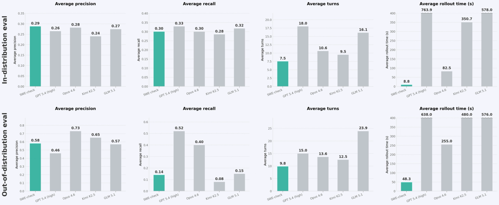
We've partnered with Applied Compute to put this to the test by collaborating to RL-train a bug detection model. The result is SWE-check, which matches frontier performance on internal in-distribution evals (delta F1 to Opus 4.6 goes from 0.09 to 0) and makes meaningful progress on out-of-distribution evals (delta F1 to Opus 4.6 goes from 0.49 to 0.29).

While SWE-check is behind the frontier on out-of-distribution evals in terms of pure capability, its order of magnitude-faster wall-clock runtime and cheaper inference cost enable an instant and free bug detection experience not possible with frontier models. We will continue to improve this model and expect that additional work on the data generation pipeline will allow us to reduce the gap to frontier performance on out of distribution evals as well. A preview of SWE-check is available in Windsurf Next today and will be released in mainstream Windsurf soon.

Here's how we did it:

• integrating natively with the production environment during RL
• using a new technique we term reward linearization to translate our desired global metric to a sample-level reward
• introducing multiple phases of post-training to build a model that is both capable and aligned with product usage patterns

The SWE-check Agent and its requirements

The SWE-check agent analyzes the current diff and flags any bugs likely introduced by the change.

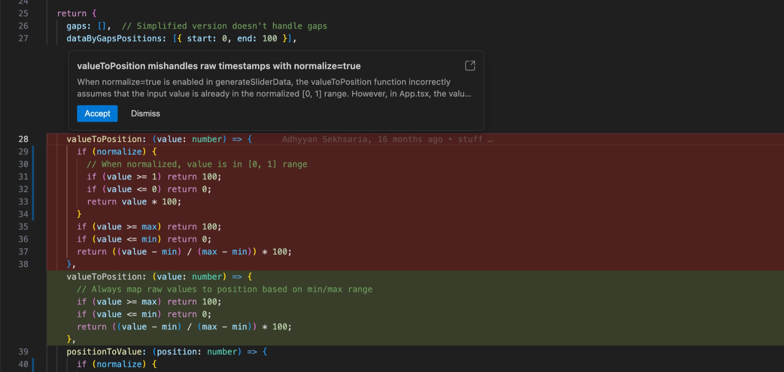
A new config flag silently switches output values from timestamps to normalized fractions. Each changed file is internally consistent, but spotting the issue requires tracing the data contract across three files to see where assumptions diverge.

This is not a typical code analysis task; unlike normal coding agents that operate in a chat interface, the SWE-check agent produces a structured output with bug descriptions and bug-fixes that render nicely in Windsurf.

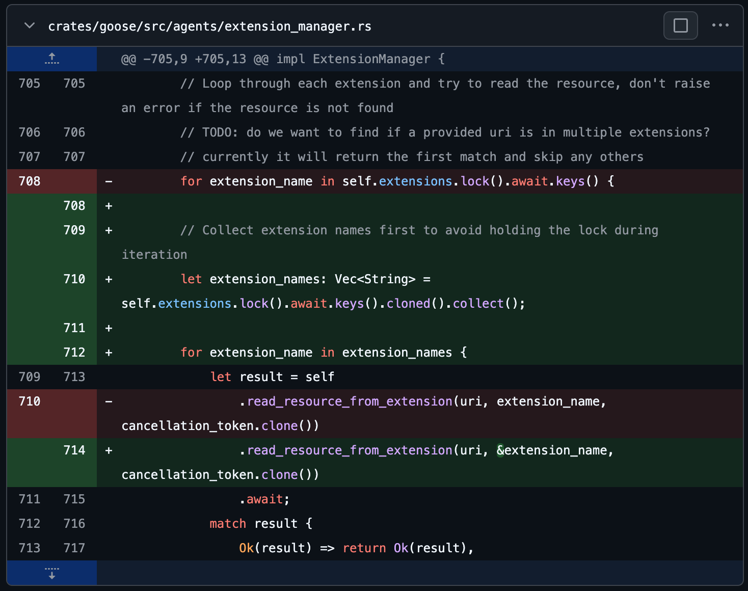
Here is an example of a ground truth bug from our training dataset, to provide a sense of the kinds of tasks the model is trained on:

Repository: block/goose

Commit: cd0b7d69

PR(s) fixing bugs that trace back to this commit: #5066

Bug 1: Concurrency & Threading - High severity (2 changes)

• Description: The code iterated over the keys view returned by self.extensions.lock().await.keys() while holding the extensions mutex guard across the iteration. The loop body then awaited a call to read_resource_from_extension, which itself may attempt to lock the same self.extensions mutex. Holding a mutex guard across an await that leads to re-lock attempts causes a deadlock, since the original guard is not released before the re-lock is requested. This manifested as the extension manager hanging when trying to read resources from extensions.
• Fix: Before iterating and awaiting into extension-specific logic, the code now collects the extension names into an owned Vec<String> by cloning the keys while holding the lock and then immediately releases the lock. The subsequent iteration runs over the collected names (no mutex held), and calls into read_resource_from_extension with a reference to each name. This prevents holding the extensions mutex across awaits and eliminates the reentrant lock attempt that caused the deadlock. A short explanatory comment was also added above the collection to document the reason.
• Ground truth bug-fix:

During training, the model starts inside a sandbox with the repo checked out to the source commit, and then its job is to output bugs that it identifies with descriptions along with bug-fixes. These bugs are compared to the ground truth bugs for that source commit.

The agent also needs to be near-real time and keep users in flow, avoiding at all costs what we call The Semi-Async Valley of Death. Fortunately, inference providers like Cerebras allow for thousands of tokens of dense intermediate thinking to happen before the final output in a matter of seconds.

At the same time, the model needs to be extremely high-quality, reliably finding subtle bugs when they exist while also not annoying the user with silly non-bugs. Before deciding to proceed with RL training, we had our colleagues dogfood various off-the-shelf frontier models, both open-source and closed-source, in the SWE-check harness. They found that frontier models that met the quality bar were too slow and expensive for on-demand bug detection in the IDE. This motivated RL-training an open-source model to be extremely specialized – fast and capable – on this task.

We ran two primary evals:

• in-distribution eval that was a random subset of the tasks generated in our data pipeline, held out from the other tasks making up the training distribution.
• out-of-distribution eval that was a collection of bugs collected internally at Cognition in the Cognition codebase and fully held-out during the training process.

Here is how the final trained model performed compared to frontier closed- and open-source models:

Training with production settings

A smaller, faster, and cheaper model trained to be a specialist can be brought to the frontier performance on its “spike” (i.e. its area of specialization). To deliver the best possible results on all three axes for our chosen spike, the SWE-check task, we therefore had to replicate the actual environment where our model would be served in production. This would ensure that any gains observed in training translate directly to an improved end-user experience in the Windsurf IDE.

To that end, we replicated the toolset available in the Windsurf harness in the training sandbox. We also curated a dataset with diverse bug types over many programming languages, and we iterated on the dataset together to ensure that the distribution was representative of what was expected in production.

We also worked extensively on aligning the training reward with user behaviors during dogfooding trials of early versions of the SWE-check agent. For example, we looked at statistical data on how long it took for users to switch off of SWE-check after invoking it (more on this in the next section).

Finally, and we think most importantly, we iteratively trained several models and built a tight feedback loop with dogfooding. Although we invested a lot of effort into training models against a reward function, ultimately human taste and how the agent feels to actually use while working is what matters most. People dogfooding the agent gave us extremely valuable feedback on every iteration.

For example, in one of the iterations, we received feedback that the model would constantly report bugs where if it simply looked up the definition of one of the variables in the code block, it would know the code block was correct. We realized the agent didn’t have access to turn-efficient tracing tools to help it look up definitions and find references, so we built and exposed these new tools in Windsurf as well as our training setup and then re-trained.

The key takeaway from the specialization process is that feedback from production directly drives iterations on the training runs. Everything that goes into the model training run has its roots traced directly back to some aspect of the production environment or feedback from real users.

How we designed the reward function

The reward used in post-training determines the model’s behaviors. Our technical report focuses on two key ideas:

• Reward linearization to provide a sample-level reward which serves as a proxy for hill-climbing the population level statistic. We take a global metric that is representative of user preferences, and convert it into a reward that can be assigned to each individual sample.
• Two-phase post-training to first maximize capability and then align the model to product usage patterns by reducing latency. We found that splitting post-training into these phases yielded a stronger model than simply training against one reward function that captures both capability and usage patterns.

Reward linearization

We begin by formalizing the training setup. Each rollout τ has its own set of ground truth bugs (possibly 0). We score a set of predicted bugs as follows:

1. We first check if the bugs are scoped correctly with a simple LLM-judge pass — if any bug in the list is actually a conglomerate of two different issues, we set the score to 0.
2. We then check if each of the predicted bugs in the list matches one of the ground truth bugs.
3. The results of these checks allows us to compute a sample-level precision and recall, which we define as P(τ) and R(τ). These should always be numbers between 0 and 1. We handle edge cases as follows:
   1. if there are no predicted bugs and no ground truth bugs, we set the precision and recall to 1
   2. otherwise, if exactly one of the predicted bugs and ground truth bugs lists is empty, then we set the precision and recall to 0

How do we aggregate these scores over many samples? There are two reasonable ways to go about this:

• We could aggregate a global total count of true positives (TP), false positives (FP), and false negatives (FN) to compute a global precision and recall, then combine them into an f_β score.
• We could average P(τ) and R(τ) over the samples to get an average precision and an average recall, then combine them into an f_β score.

Since we would not want to bias the model to be disproportionately good at examples where there are a lot of ground truth bugs (at the expense of poor performance on examples where there are few / no ground truth bugs), we opt for the second choice.

🚨 Choice of β: Early iterations of the model used β=1 and produced many false positives, flagging many benign diffs as bugs during dogfooding. To mitigate this, we decided to switch to β=0.5, emphasizing precision.

We define R_pop = E_τ[R(τ)] and P_pop = E_τ[P(τ)]. We ultimately want the model to increase the metric

Given this global metric, what should our sample level reward then be? A key observation is that we cannot directly use

because averaging f_β(τ) does not yield f_β. This motivates our idea of reward linearization, where we compute a first order approximation of f_β in terms of P_pop and R_pop, so that the averaging actually does work out!

Since we have a good sense of the initial values of P_pop, R_pop (call these initial values P_pop,init and R_pop,init), and the initial distribution of TP/FP/FN rates, then we can approximate the f_β value with a suitable first order linear approximation in P_pop and R_pop:

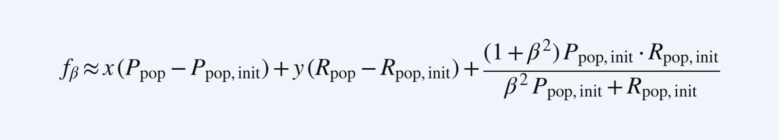
🚨 It is important that the first order approximation is done with awareness of the initial values of the TP/FP/FN rates. In our runs, the changes in TP/FP/FN rates did not change the resulting slopes drastically over the course of the run so we used a fixed linearization; our method could be generalized by recalibrating the first order approximation during training if some of the initial values deviate too much.

Then a valid sample-level reward function (since it averages to the desired f_β approximation above) would be

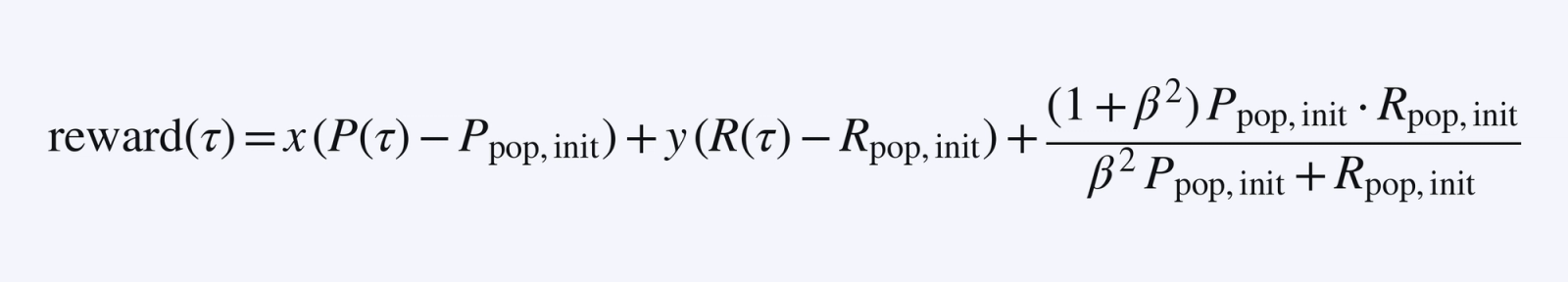
In fact, we can translate/scale the reward function, so we can force y=1 and remove all the constant terms. In our case we ended up using the sample level reward reward(τ) = ½·P(τ) + R(τ). A model that receives the reward reward(τ) for each sample will end up climbing the global f_β metric, as desired!

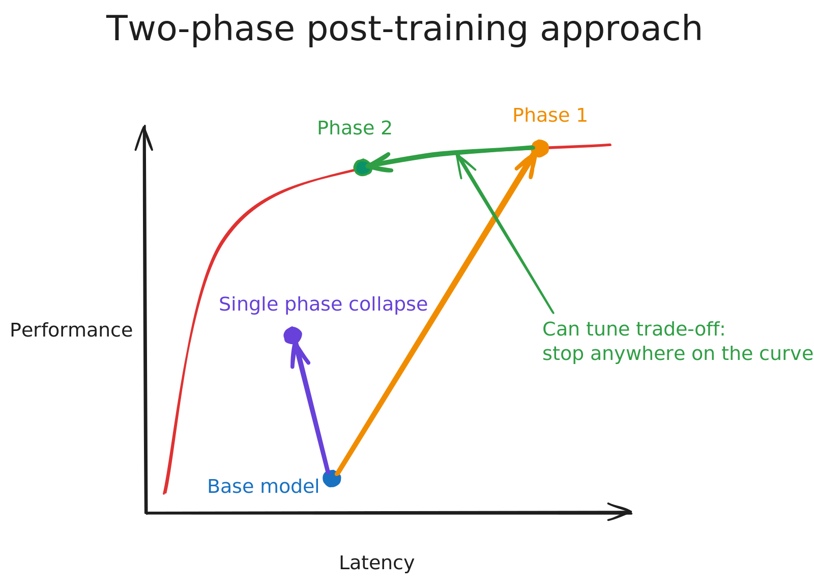
Two-phase post-training

Our goal was to train a model with frontier performance that had a much better latency profile. We found that the most effective training approach split the process into two distinct phases. The two phases differ only in the reward function, with the rest of the training setup remaining exactly the same.

1. Capability maximization: The reward function is the base reward function which we computed in the reward linearization section. By climbing this reward, the model focuses purely on maximizing bug detection skill and is not penalized for incremental latency. Capability maximization was the bulk of the overall training process.
2. Product alignment: The reward function is the base reward function plus an additional “latency penalty”. To compute the latency penalty, we first estimated the latency of the rollout using the number of completion tokens and tool-calling turns. Then, we observed the statistical distribution for how long it takes users to switch off of SWE-check after invoking it using dogfooding data from an early internal version of the SWE-check agent.

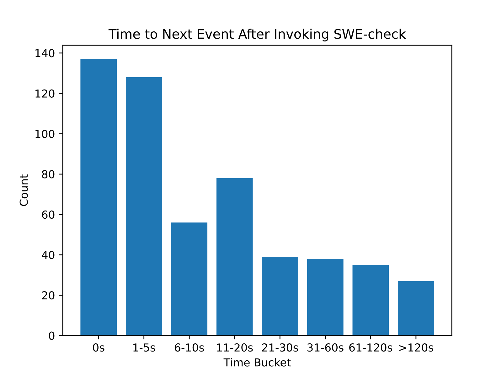
This distribution was effectively a proxy for how much time we had to keep users in-flow. We then computed the CDF of this distribution and used it to define a penalty that scales with estimated latency. The CDF at a given time tells us what fraction of users would have already moved on by then.

We normalized the penalty so that it starts at 0 for instant responses and is 1 at the tail, then linearly interpolated between bucket midpoints.

The product alignment reward pushed the model to shed redundant tokens and improve parallel tool-calling, while not sacrificing performance for latency beyond what was necessary for user experience. Product alignment was a much shorter phase than capability maximization in terms of training compute.

This two-phase approach outperformed the alternative of training with a single combined reward function from the start. When capability and product constraints were optimized simultaneously, the model tended to converge on local optima: for instance, learning to be extremely fast but producing shallow analysis that satisfied the latency target but missed real bugs. Separating the phases allowed the model to first develop genuine understanding of the task, then learn to compress that understanding efficiently.

Additionally, in the second phase of post-training we observed:

• Initially, the model had minimal performance degradation while the latency penalty was reduced;
• Then, the model’s performance began more noticeably declining as the latency penalty continued to decrease.

The second phase therefore is a tunable knob which we can use to choose exactly the performance-latency profile that fits our use case best. In our case, we selected the point on this Pareto frontier based on product usage patterns, as discussed earlier.

Conclusion

To recap, model specialization is a powerful tool to approach frontier performance with a better latency, cost, and user experience profile that is deeply aligned with the product feature.

Integrating natively with the harness ensured our training gains would reflect in production. Frequent dogfooding trials allowed us to quickly translate user feedback into changes in the training recipe. Using reward linearization allowed us to effectively boil a production performance metric down to the sample level for training. Splitting post-training into multiple phases empowered us to balance two different goals – capability in the core task and product latency requirements – in our model training.

There is still meaningful room for improvement in the final model – although it is on the Pareto frontier, it is not categorically the most capable model on this task. The training recipe discussed has proven to hill-climb well on both in-distribution and out-of-distribution evals, and with a broader data mix and improved base models, we expect continued performance gains over time.

You can try a preview of SWE-check today in Windsurf Next using the cmd+U shortcut. It will be available in Windsurf soon.